Calculating Gravity - Gulf Coast Data Concepts

Introduction

Occasionally, it’s a good idea to check some of the fundamental laws of physics for validity. You never know if those physicists made a mistake or if the nature of the universe recently took a turn for the worse. Here, a USB accelerometer data logger made by Gulf Coast Data Concepts was used to determine the periodicity of a simple gravity pendulum and to calculate acceleration of gravity. The test determined the local gravity as 32.24082 ft/sec², which is within 1% of Earth’s nominal gravity of 32.1740 ft/sec². The results indicate that gravity does, in fact, still work, and all is well in the universe.

Objective

The test analyzed data collected from a GCDC accelerometer data logger to calculate the acceleration of gravity using a simple gravity pendulum.

Procedure

Equipment

Description	Quantity	Comments
Weight	1	Standard 2lb exercise weight
Eyehook	1	Available at most hardware stores
X16-D USB Accelerometer (or HAM-x16)	1	Purchase online from GCDC
High strength fishing line	–	This experiment uses Berkley Fireline. Other string-like materials would be fine, but note that regular string might stretch or twist.
Electrical Tape	–	Any tape will suffice
Measuring Tape	1	12′ long retracting tape measure

Materials and Equipment List

Logger Configuration

;X16-1E configuration
    ;set sample rate
    ;available rates 12, 25, 50, 100, 200, 400
    samplerate = 100
    ;record constantly
    deadband = 0
    deadbandtimeout = 0
    ;set file size to 5 minutes of data
    samplesperfile = 30000
    ;set status indicator brightness
    statusindicators = High
    ;rebootOnDisconnect

Steps

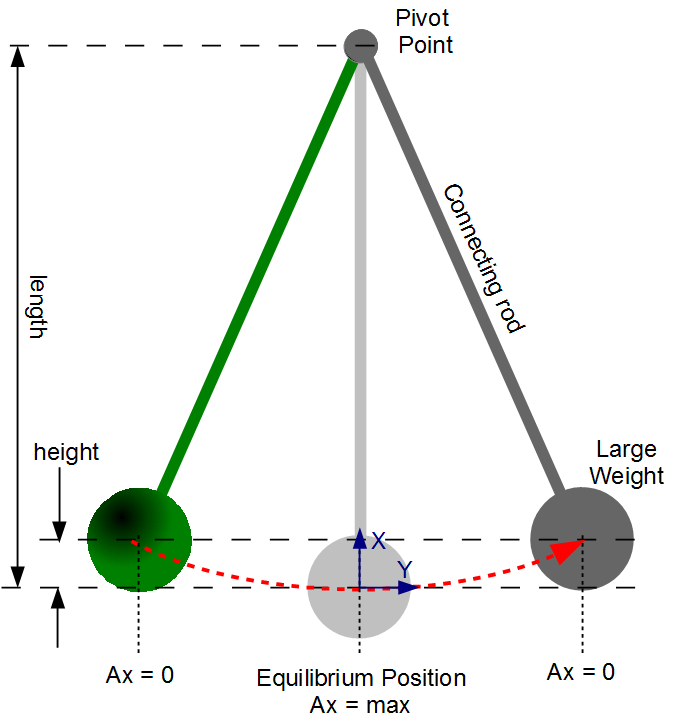
For this experiment, a small dumbbell weight served as the pendulum bob, and an eyehook attached to a door frame worked as the pivot point. The effective length of the pendulum arm is the distance between the pivot point and the center of mass. The string is negligible weight, so the center of mass is located at the middle of the dumbbell.

The following steps outline the procedure for the experiment setup:

Attached eyehook to the top of a standard door frame.
Tied fishing line around weight.
Taped the logger onto the weight with the On/Off button facing up for easy access.
Threaded the fishing line through the eyehook and knotted it so that the weight hovered several inches above the ground. Note that the weight does not have to hang evenly, as this will not affect the outcome.
Measured the length of the fishing line from the knot at the eyehook to the middle of the weight. This distance is the effective length of the pendulum.

The following steps outline the procedure for the experiment:

Turned on the logger, pulled the weight back approximately 18 inches while keeping the string taut, and released, causing the weight to swing. Note that the weight does not have to swing in a straight motion, as the analysis procedure takes this into account.
Allowed the pendulum to swing for 5 minutes before stopping it and turning off the logger.

The analysis was performed using “R”, which is a free open source mathematics package available at www.r-project.org. An R script called “pendulum_analysis.r” was developed to analyze the test data from the accelerometer data logger and determine the time period of the pendulum (see Appendix A for full script).

The script converted the accelerometer time series data to the frequency domain using a Fast Fourier Transform (FFT) function. Consecutive segments of data were taken from the file and processed through the FFT until the entire file was analyzed. All the FFT results were averaged together into a single spectral plot of acceleration versus frequency. This method averaged out intermittent changes in behavior and increased the signal-to-noise ratio of the results.

The plot illustrated the dominant frequency of the swinging pendulum, which is due to the maximum acceleration in the x-axis as the pendulum swings past the vertical position. A complete swing includes the pendulum passing through the vertical position twice. Therefore, the swing frequency of the pendulum is half the dominant frequency, and the swing period is the inverse of the that frequency.

Results

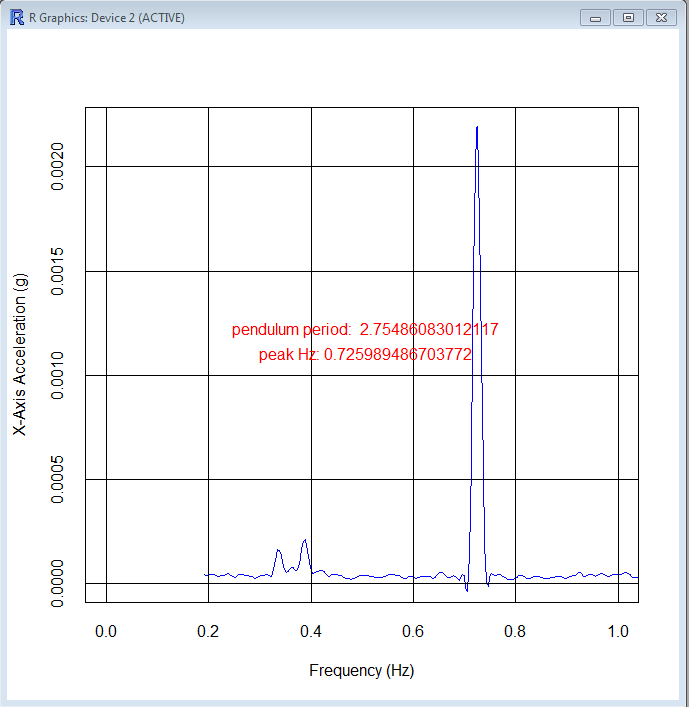
R automatically plotted the results of the analysis and determined the dominant frequency to be 0.725989 Hz. There are two acceleration peaks per cycle since the pendulum swings past center twice. Therefore, the frequency of the pendulum is half that of the FFT result, or 0.3629945 Hz. The resulting pendulum period was 2.75486 seconds.

R calculated gravity using the 2.75486 second period and Equation 2. Gravity equaled 32.24082 ft/sec^2.

Plots

Discussion

Using R to determine acceleration due to gravity resulted in a very accurate assessment of Earth’s gravity. The test determined the local gravity as 32.24082 ft/sec^2, which is within 1% of Earth’s nominal gravity of 32.1740 ft/sec^2.

Conclusion

Calculating the acceleration of gravity to within 1% of actual using such a crude experiment is impressive. Furthermore, we can conclude that gravity still works, and all is well in the universe (at least in Waveland, MS).

Supporting Files

GCDC-TR003_Calculating_Gravity_with_Pendulum Download